Obtaining a MUSE image with a given bandpass
The photometry fitting algorithms are designed to compare MUSE and HST images that have similar wavelength sensitivity curves. Each MUSE observation generates a cube of 3681 narrow-band images, at wavelength intervals of 1.25 angstroms, whereas each HST image has an effective bandwidth of hundreds of angstroms and a non-flat wavelength response curve. To generate a MUSE image that has the same spectral characteristics as an HST image, the narrow band images of the MUSE cube have to be combined, weighted by the spectral-sensitivity curve of the HST image. This can be done using the make_wideband_image script.
The make_wideband_image script takes a
MUSE cube and a filter curve and generates a wide-band MUSE image that
has the spectral response of the filter curve. A function that does
the equivalent operation is also available, called
imphot.bandpass_image()
The arguments of the function can be obtained by running it with the
-h option:
% make_wideband_image -h
usage: make_wideband_image [-h] [--prefix [output-prefix]] [--quiet]
                           [--wave_units [wavelength-units]]
                           filter_curve muse_cubes [muse_cubes ...]

positional arguments:
  filter_curve          The filename of the wavelength sensitivity curve of
                        the camera. The file should be a text file with two
                        columns of numbers. The first column are the filter-
                        curve wavelengths, and the second are the
                        corresponding sensitivities, which should be unit-
                        less. The sensitivities will be normalized by the area
                        under the sensitivity curve, so only their relative
                        values are important.
  muse_cubes            The filenames of a MUSE cubes to be processed.

optional arguments:
  -h, --help            show this help message and exit
  --prefix [output-prefix]
                        When this option used, it specifies a prefix to use
                        when constructing the names of the output FITS files.
                        The output files are then named,
                        "<prefix>_<input_name>", where <prefix> is the
                        specified string, and <input_name> is the base-name of
                        the input cube, but with the first instance of either,
                        "datacube" or "cube", replaced with "image". When this
                        option is omitted, the prefix defaults to the base-
                        name of the filter file.
  --quiet               Suppress the messages that report each step as it is
                        performed.
  --wave_units [wavelength-units]
                        DEFAULT=Angstrom. The units of the wavelengths in the
                        file of sensitivity versus wavelength. If this option
                        is not specified, angstroms are assumed.
%
For example, the following command takes the cube of a MUSE observation of the MUSE UDF08 field, and creates an image that has the same spectral characteristics as the HST ACS with the HST F606W imaging filter:
% make_wideband_image wfc_F606W.dat DATACUBE-MUSE*.fits
Reading filter: wfc_F606W.dat
Reading cube: DATACUBE-MUSE.2014-09-21T07:12:55.019.fits
Computing the output image.
[WARNING] 1.1% of the integrated filter curve is beyond the edges of the cube.
Writing image to: wfc_F606W_IMAGE-MUSE.2014-09-21T07:12:55.019.fits
WARNING: VerifyWarning: Card is too long, comment will be truncated. [astropy.io.fits.card]
Reading cube: DATACUBE-MUSE.2014-09-21T07:39:42.019.fits
Computing the output image.
[WARNING] 1.1% of the integrated filter curve is beyond the edges of the cube.
Writing image to: wfc_F606W_IMAGE-MUSE.2014-09-21T07:39:42.019.fits
%
Note the warning message that says that 1.1% of the integrated filter curve lies beyond the edges of the cube. The reported number is the fraction of the area under the filter curve that is outside the wavelength coverage of the MUSE cube. The warning can safely be ignored if the percentage is low, but larger percentages will yield a wide-band image whose spectral response curve is not a good approximation of the filter curve, and the photometry fits will yield large residuals for sources that have significant spectral indexes.
Also note that the name of each output file is based on the name of the corresponding input CUBE. By default the output filename is the concatenation of the filter-curve filename (minus its extension), and the input CUBE filename. To avoid creating a filename that implies that a cube has been created, any initial instance of the word datacube or cube in the output filename is automatically replaced with the word, image.
Performing the same operation from a python script
Arbitrary python scripts can obtain the same result as the make_wideband_image script as follows:
from mpdaf.obj import Cube
import numpy as np
cube = Cube(hst_filename)
w, s = np.hsplit(np.loadtxt(bandpass_filename, usecols=(0,1)), 2)
imphot.bandpass_image(cube, wavelengths=w, sensitivities=s, unit_wave=u.angstrom)
HST filter curves
Filter curves for HST filters that overlap the wavelength coverage of the MUSE cube, can be found at the following URL:
For HST UDF observations, the pertinent filters are the following ACS WCS filters:
Filter name |
Filter overlap |
Filter curve |
|---|---|---|
F606W |
99% |
|
F775W |
100% |
|
F814W |
96% |
|
F850LP |
73% |
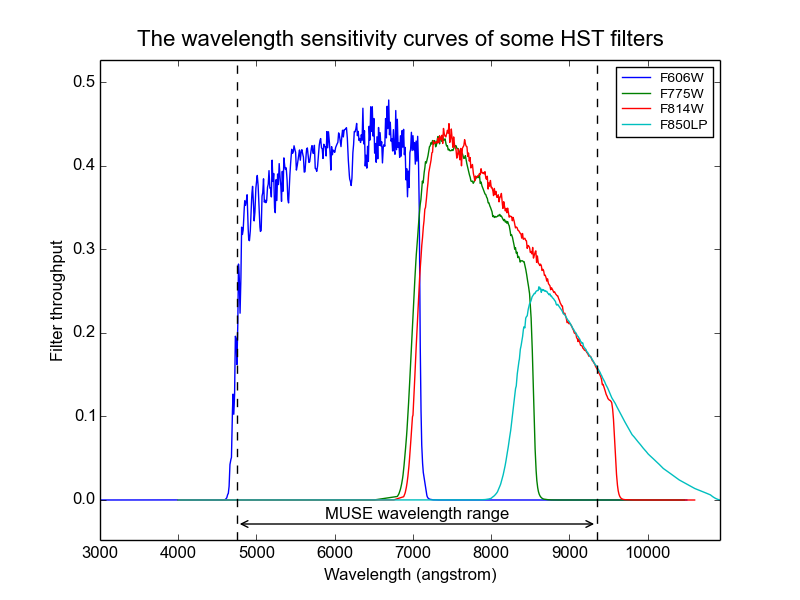
The filter overlap column indicates how much of the integrated bandpass lies within the MUSE wavelength range. The response curves of these filters are shown in the following figure. Note the two vertical lines that delimit the wavelength coverage of MUSE cubes.