A tutorial on photometric parameter fitting
The following tutorial will describe the steps needed to fit the photometric parameters of a MUSE cube. The following steps will be elaborated.
1: Downloading a suitable HST observation
First an HST image is downloaded that incorporates the majority of the area covered by the MUSE observation, and that has a spectral response curve that lies mostly within the wavelength coverage of the MUSE cube.
2: Extracting a suitable image from the MUSE cube
Next an image is extracted from the MUSE cube that has the same spectral response curve as the HST image.
3: Resample and rescale the HST image
Next the HST image is resampled onto the pixel grid of the MUSE image obtained in step 1, and its fluxes are rescaled to have the same units as the MUSE image.
4: Perform a global image fit for the photometric parameters
The photometric parameters of the MUSE image are first fitted using the default global image fitting algorithm.
5: Ignoring a problematic star while fitting
In step 4, the plotted residuals of the fit show that one star in the image does not fit very well, so in this step, to improve the fit, the fitting script is run again, but this time a circular region of pixels around the star are excluded from the fit.
6: Performing a fit to a bright star
As an alternative method of handling the effect of a bright star, this step performs the fit on a small area of the image that includes the star, and also performs star profile fits, to obtain independent estimates of the photometric parameters.
Downloading a suitable HST observation
A prerequisite of the fitting procedure is that there be an HST WFC ACS observation of the same region as the MUSE cube, taken through an HST imaging filter that significantly overlaps with the MUSE wavelength coverage. The chosen HST image should be as published by STSCI. Specifically it should still be calibrated in electron/s, and its pixel size should be on the order of 0.03 to 0.06 arcsec, depending on which version of the ACS was used, and whether or not the image drizzling was used.
This tutorial will fit for the photometric parameters of an observation of the MUSE UDF04 field. This field is a subset of the HST Ultra Deep Field, and corresponding HST observations of this field are available at the following web page:
The above page lists images taken through a number of different imaging filters. From section, HST filter curves, we know that the filters, F606W, F775W, F814W and F850LP, significantly overlap with the MUSE coverage.
The web-page also provides equivalent images that have 30mas pixels and 60mas pixels. It is always best to choose the highest resolution image that is available. The reason is that when an image is resampled to a lower resolution, a decimation filter is applied to avoid aliasing, and this changes the size and profile of the PSF. The photometry fitting program is very sensitive to the PSF profile of the HST image, so this can degrade the results. Note that the fitting program has been optimized for HST images with 30mas pixel sizes, so this is the best resolution to obtain if possible.
For the tutorial, the following image is downloaded, which has 30mas pixels, and was taken through the F775W filter:
hlsp_xdf_hst_acswfc-30mas_hudf_f775w_v1_sci.fits
Extracting a suitable image from the MUSE cube
The fitting procedure needs a MUSE image that has the same spectral
response curve as the chosen HST image. In this demo, the spectral
response of the HST image is that of the F775W filter of the HST Wide
Field Camera. The following example, which is run from a normal shell
prompt, uses the make_wideband_image
script to extract an image of this response curve from a MUSE cube
called udf04_cube.fits:
% make_wideband_image wfc_F775W.dat udf04_cube.fits
Reading filter: wfc_F775W.dat
Reading cube: udf04_cube.fits
Computing the output image.
Writing image to: wfc_F775W_udf04_image.fits
%
On a single 2.4GHz CPU this took one minute to run. Beware that this script requires a lot of memory. This is because MUSE cubes are large, and MPDAF reads the whole cube into memory. For example, the above process showed peak memory usage of 22GB of memory.
Resample and rescale the HST image
The fitting procedure also requires that the reference HST image be resampled onto the same pixel coordinate grid as the MUSE image. In the following example, the regrid_hst_to_muse script is used to resample the HST image that was downloaded in step 1. The MUSE image that was extracted in step 2 is also used to indicate the desired pixel grid. In addition to resampling the the HST image, this script also changes its units from electron/s to the flux units of the MUSE image:
% regrid_hst_to_muse --field UDF04 wfc_F775W_udf04_image.fits hlsp_xdf_hst_acswfc-30mas_hudf_f775w_v1_sci.fits
Reading MUSE image: wfc_F775W_udf04_image.fits
Reading HST image: hlsp_xdf_hst_acswfc-30mas_hudf_f775w_v1_sci.fits
WARNING: MpdafUnitsWarning: Error parsing the BUNIT: 'ELECTRONS/S' did not parse as unit: At col 0, ELECTRONS is not a valid unit. Did you mean electron? [mpdaf.obj.data]
Resampling the HST image onto the MUSE pixel grid.
Changing the flux units of the HST image to match the MUSE image
Writing the output file: hst_F775W_for_UDF04.fits
%
Note that the warning message about electrons/s units can safely be ignored. This comes from the astropy.units module when it reads the FITS header of the HST image. The script knows what the actual units are in HST images, so it ignores the claimed units, and rescales the fluxes from HST electron/s units to physical units without consulting the incorrectly parsed units from the header.
For reference, this process took 30 seconds on a single 2.4GHz CPU, and had a peak memory usage of 1.7GB.
Perform a global image fit for the photometric parameters
At this point, we now have a pair of HST and MUSE images that can be used to fit for the photometric parameters of the MUSE image. We start by performing a fit using default parameters of the fit_photometry script. We also use the –display option to request that a plot of the fit be shown:
% fit_photometry hst_F775W_for_UDF04.fits wfc_F775W_udf04_image.fits --display
# MUSE observation ID              Method    Flux    FWHM    beta      Flux  x-offset  y-offset   RMS
#                                           scale     (")            offset       (")       (")  error
#--------------------------------- ------  ------  ------  ------  --------  --------  --------  ------
             wfc_F775W_udf04_image  image  0.9819  0.5697  2.5000   0.04191  -0.00188  -0.01732  0.0699
%
With the default arguments, this reports a summary of the fitting
photometric parameters. The addition of the --verbose option could
alternatively be used to list many more details of the fit, including
uncertainties, reduced chi-squared etc.
The reported beta value is precisely 2.5 because by default this
parameter is fixed in the fit to that value. This is done because
there is some degeneracy between this parameter and other parameters
in the fit, and it is easier to obtain a smooth trend in the fitted
FWHM value versus wavelength if the beta value is constrained to the
same value in all fits. The restriction can be removed by adding the
option --fix_beta=none.
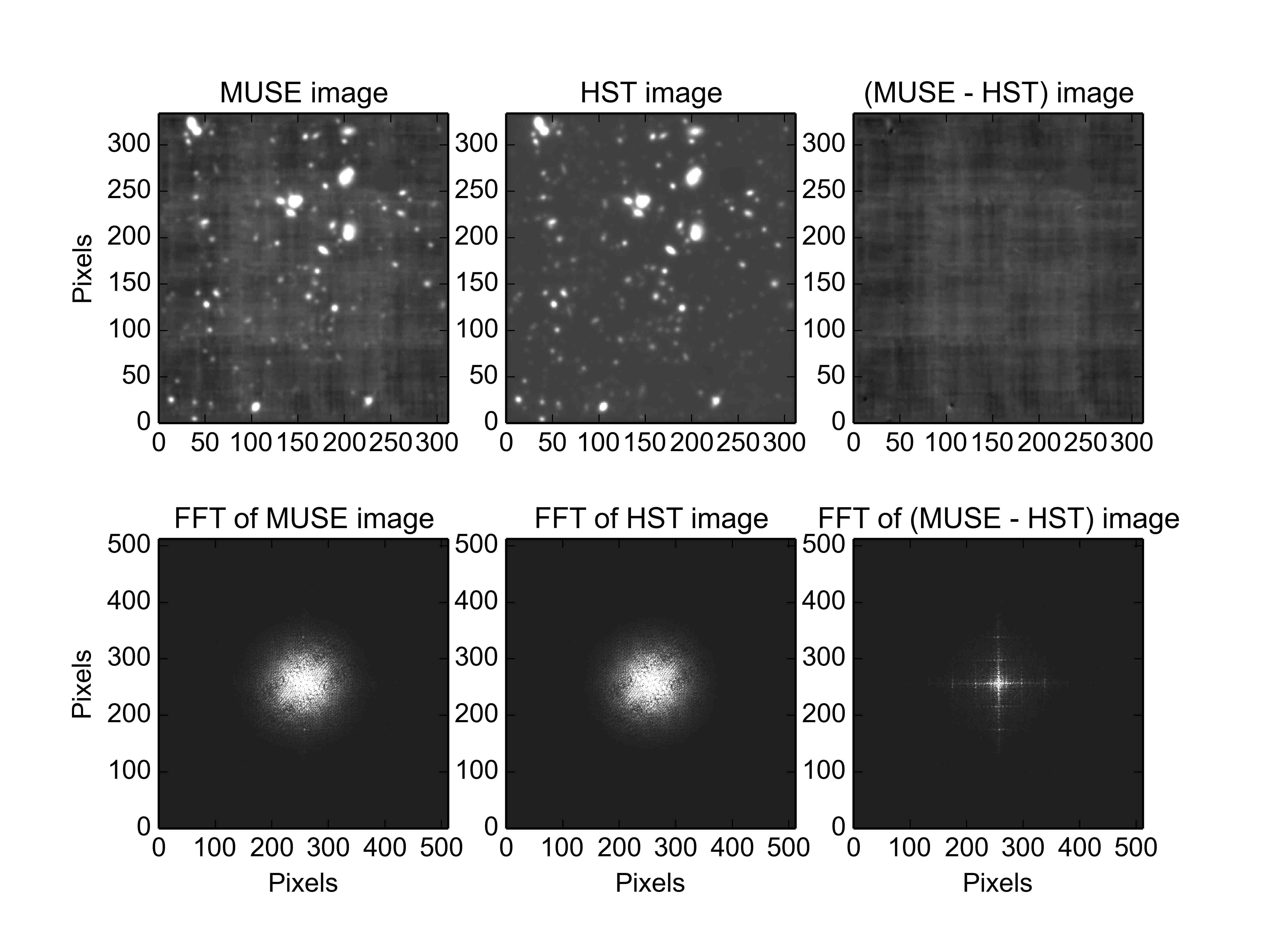
The following plot was generated by the above example. The plot was saved to a JPEG file by running the example again, this time with the –hardcopy option.

The image shown in the top-left corner of the plot is the input MUSE image, after it has been given a mask that matches that of the HST image, and after it has been convolved with the antialiasing filter that was used when resampling the HST image in step 1. Under the MUSE image is its Fourier transform, which is where the fitting procedure operates.
The middle of the top-most plots is the best-fit simulation of the MUSE image based on the HST image. This is the HST image after it has been convolved with the best-fit MUSE PSF, scaled and offset by the best-fit calibration factors, and shifted in position by the best-fit x and y position offsets. Ideally it would be identical to the MUSE image.
The image plotted in the top-right corner of the plot, is the difference between the two images to the left of it. In other words, this is an image of the residuals of the photometric fit. Ideally it would be an image of the background noise and instrumental defects. Indeed, most of the residual image appears to be an image of the systematic stripes that are seen in the background of the original MUSE image. However there is also a bright spot near the top-left corner of the residual image, which turns out to be the residuals of a bright star. This is a common occurrence for the following reasons.
The global image fitting algorithm works by assuming that the only difference between two observations of the same patch of sky, are differences caused by seeing, pointing errors and calibration errors. However if the HST and MUSE observations are performed at different times, then this assumption can be broken by any variable sources in the field, and more importantly by stars with significant proper motion. This is the explanation of the residuals in the above image. Looking closely at the residual plot, one can see that the residuals are bright on the left and dark on the right, implying that the star moved leftwards, in this case by about a 0.2 arcsecond pixel.
Ignoring a problematic star while fitting
In the previous step, the global image fit revealed a star that didn’t fit very well, because it had moved slightly between the HST and MUSE observations. In this case the problematic star didn’t seem to bias the fit significantly, because all of the other sources were well subtracted. However when a field contains one or more bright stars that move by even a fraction of a pixel between the HST and MUSE observations, the global fit can be badly affected. There are a couple of ways to handle this, as described in this and the next steps of the tutorial.
One way to handle the problem of a bright star with high proper
motion, is to mask a small area of the image where the star is, so
that it doesn’t contribute to the fit. This can work well in fields
that contain lots of sources after the problematic ones have been
removed. The way to do this is to use the –regions
option with a ds9 region file that defines a small region to be
excluded around the star. We will use the region file,
exclude_udf_stars.reg,
which includes the following lines, among others:
fk5
-circle(53.148540, -27.770139, 2.0")
The minus sign that precedes the circle line, indicates that the
region is to be excluded from the fit. The first two numbers within
the brackets are the fk5 Right Ascension and Declination of the center
of the circle in degrees, and the final number is the radius of the
circular region. In this case the radius is followed by " to
indicate that it is given in arcseconds. Without this, the radius
would be assumed to be in degrees.
The
exclude_udf_stars.reg
region file also contains similar exclusion lines for stars that are
to be excluded in other UDF fields. The file was created by running
ds9 on the MUSE image and using the mouse to define circular regions,
centered on each star. The region file is passed to the
fit_photometry script, via the
–regions parameter, as follows:
% fit_photometry hst_F775W_for_UDF04.fits wfc_F775W_udf04_image.fits --regions exclude_udf_stars.reg --display
# MUSE observation ID              Method    Flux    FWHM    beta      Flux  x-offset  y-offset   RMS
#                                           scale     (")            offset       (")       (")  error
#--------------------------------- ------  ------  ------  ------  --------  --------  --------  ------
             wfc_F775W_udf04_image  image  0.9768  0.5730  2.5000   0.04169   0.01401  -0.01656  0.0675
%
The results are very similar to those of the previous step, which indicates that, in this case, the star didn’t bias the previous fit significantly. The plot this example generated, is the following:
In this image the problematic star no longer appears in either the MUSE image or the HST image, because the region-file caused a circular area there to be masked. As such it is no surprise that it is no longer visible in the residual image. Otherwise, the residual image looks about the same as before.
Performing a fit to a bright star
Another way to handle the problem of a bright star with high proper motion, is to restrict the fitted part of the image to a small region that encloses the star. This is often the best option, because the profile of a bright star should be able to provide a good fit for the photometric parameters.
In the previous step the –regions option was used to mask the area where the star was, to prevent it from biasing the fit. The –regions option could alternatively be used to mask everywhere except where the star is, by using a region file that didn’t have a minus sign before the circular region definition. However a better, and more convenient approach is to use the –star option. This takes the star position and the radius of the region around it to include in the fit, and since this is given on the command-line, there is no need for a region file:
% fit_photometry hst_F775W_for_UDF04.fits wfc_F775W_udf04_image.fits --star 53.148540 -27.770139 3.0 --display
# MUSE observation ID              Method    Flux    FWHM    beta      Flux  x-offset  y-offset   RMS
#                                           scale     (")            offset       (")       (")  error
#--------------------------------- ------  ------  ------  ------  --------  --------  --------  ------
             wfc_F775W_udf04_image  image  1.1581  0.5711  2.5000   0.08863  -0.13003  -0.02434  0.0217
             wfc_F775W_udf04_image  stars  1.2289  0.5658  2.5000   0.06651  -0.13615  -0.02581  0.0815
%
Note that this generated two lines of fitted photometric parameters. On the first line the Method column says image, which indicates that the parameters were fitted by the global image fitting algorithm. On the second line the Method column says stars, which indicates that the parameters there were fitted by fitting Moffat PSF profiles to the same star in the HST and the MUSE images, and comparing the results. In principle, if the star is bright and it really is a point source in both images, then the results of the two techniques should be the same. In this case the results are very similar, apart from a 6% difference in the fitted scale factors.
In both sets of fitted parameters, the scale factor is about 20% higher than in the previous fits that operated on the whole image. This turns out to be a typical feature of star fits. It implies is that either the fluxes of the star in the HST image are lower than expected, or that the fluxes of stars in MUSE images are larger than expected. This does not appear to be a saturation phenomenon, because it doesn’t appear to worsen with increasing stellar flux.
So far this algorithm has only been tested on fields in the HST UDF, and the HST UDF images are the accumulation of a decade of individual observations, so one possible explanation for the high scale factor for star fits, is that either proper-motion or parallax-induced motion of nearby stars in the UDF, has smeared the flux of the stars in the HST images, widening their profiles in one direction and reducing their apparent peak fluxes. There is indeed evidence for such widening along one direction when the 2D residuals of the fits to bright stars are examined closely. If this positional explanation is correct, then the increase in the scale factor on a given star should be the same at all wavelengths, and affect all MUSE images equally, so useful comparisons of the scale factor can still be made between different MUSE exposures of a field.
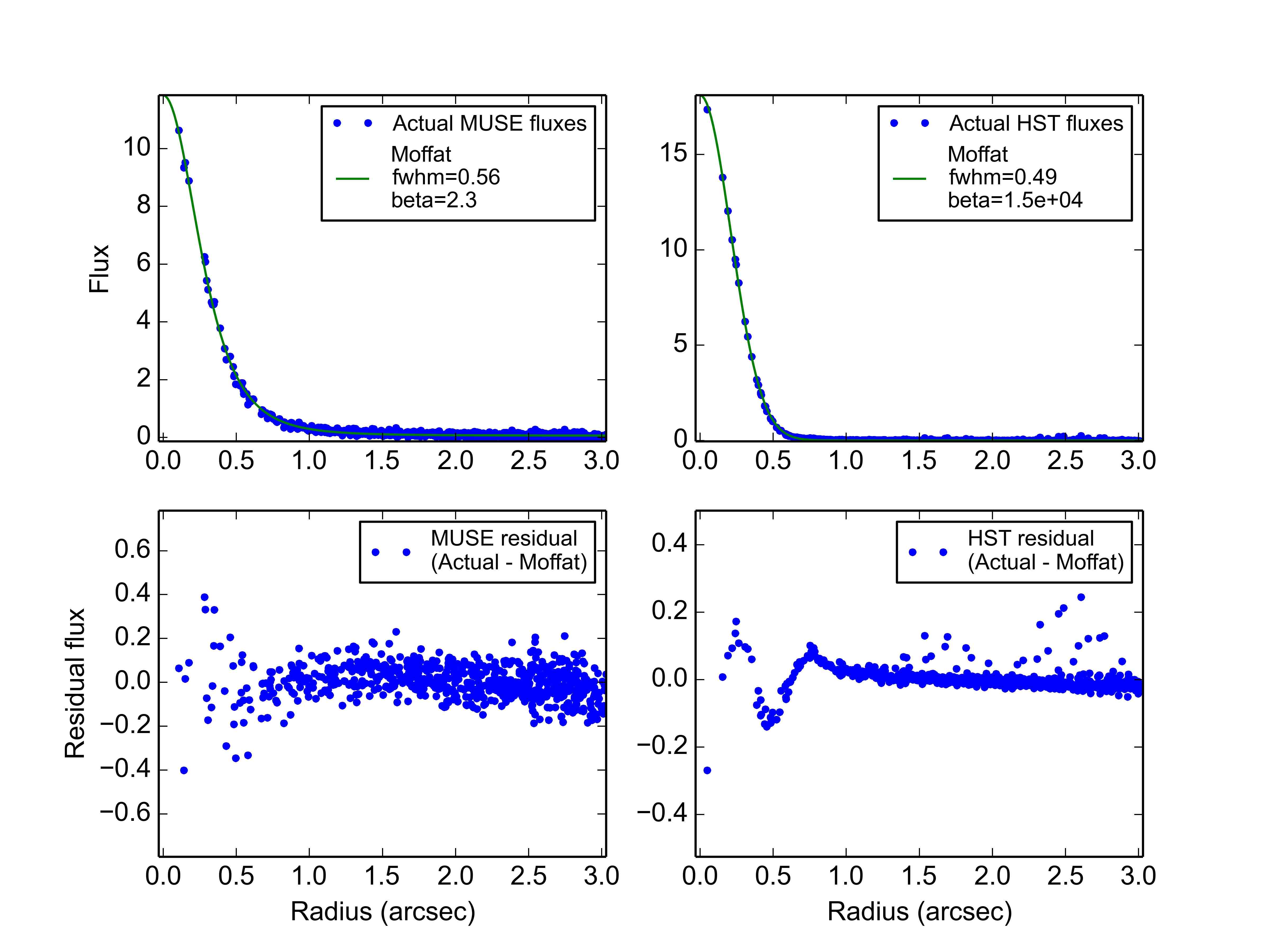
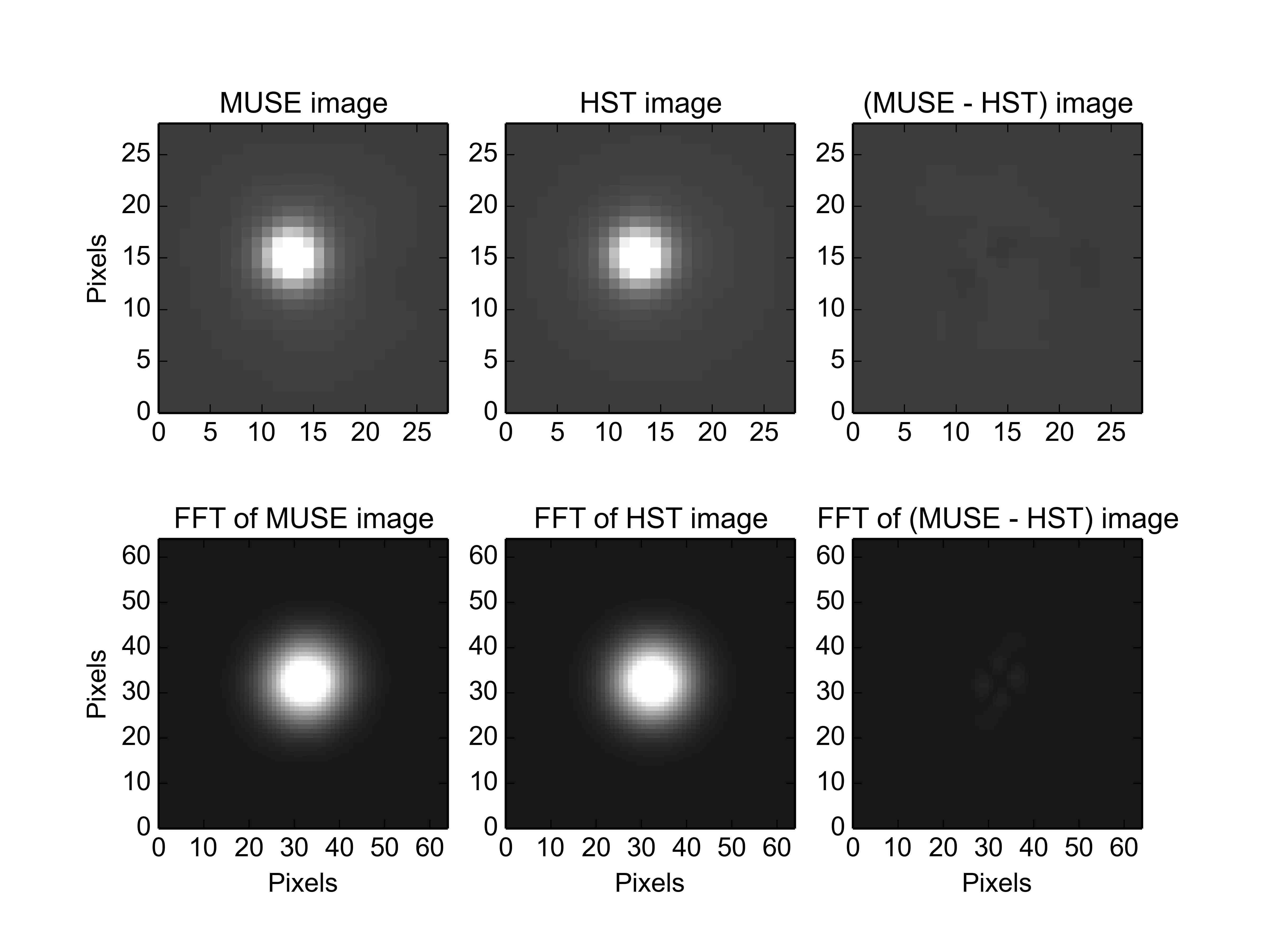
The above example generated two plot files. The first showed the result of the image fitting algorithm, showing just the small area of the image that the fit was performed on:
The second plot file shows the Moffat profile fit to the star in the MUSE image, followed by the Moffat profile fit to the star in the HST image.